2025-12-09 16:07:23

The benchmark known as "thermal bridges" is an example of an application that enables us to validate numerical simulation tools using Feel++. We have developed tests based on the ISO 10211:2017 standard (ISO 10211:2017 - Thermal bridges in building construction — Heat flows and surface temperatures — Detailed calculations, 2017), which provides methodologies for evaluating thermal bridges in building construction.

Thermal bridges are areas within a building envelope where heat flow is different compared to adjacent areas, often resulting in increased heat loss or unwanted condensation. The standard is intended to ensure that thermal bridges simulation are accurately computed. It provides reference values (and tolerance) on heat temperature and heat flux at several location of the geometry.

At the mathematical level, this application requires finding the numerical solution of an elliptic linear PDE (i.e. the heat equation). We employ a finite element method based on continuous Lagrange Finite Element of order 1,2 and 3 (denoted by P1,P2,P3). And we analyzed the execution time of the main components of the simulation.

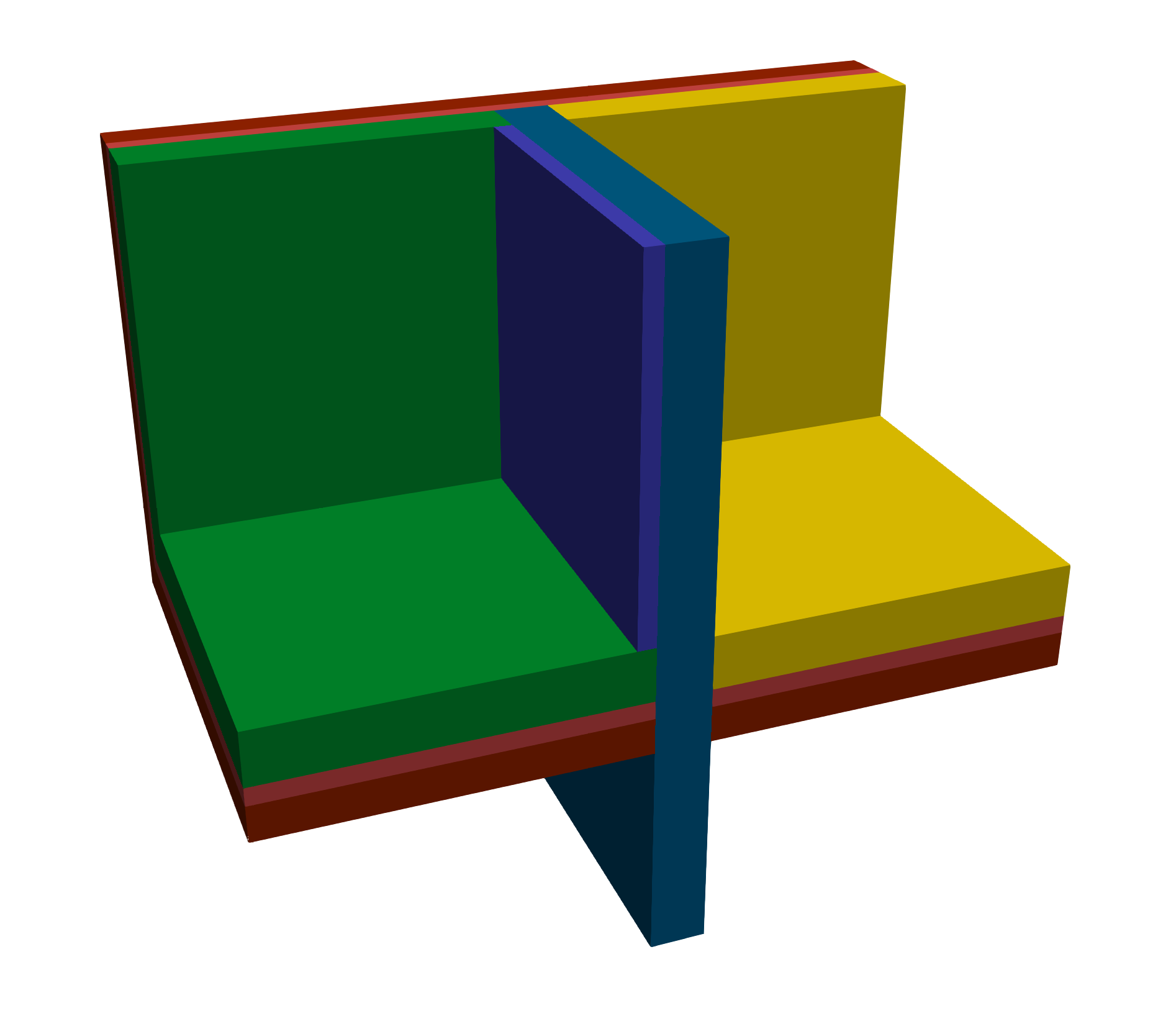
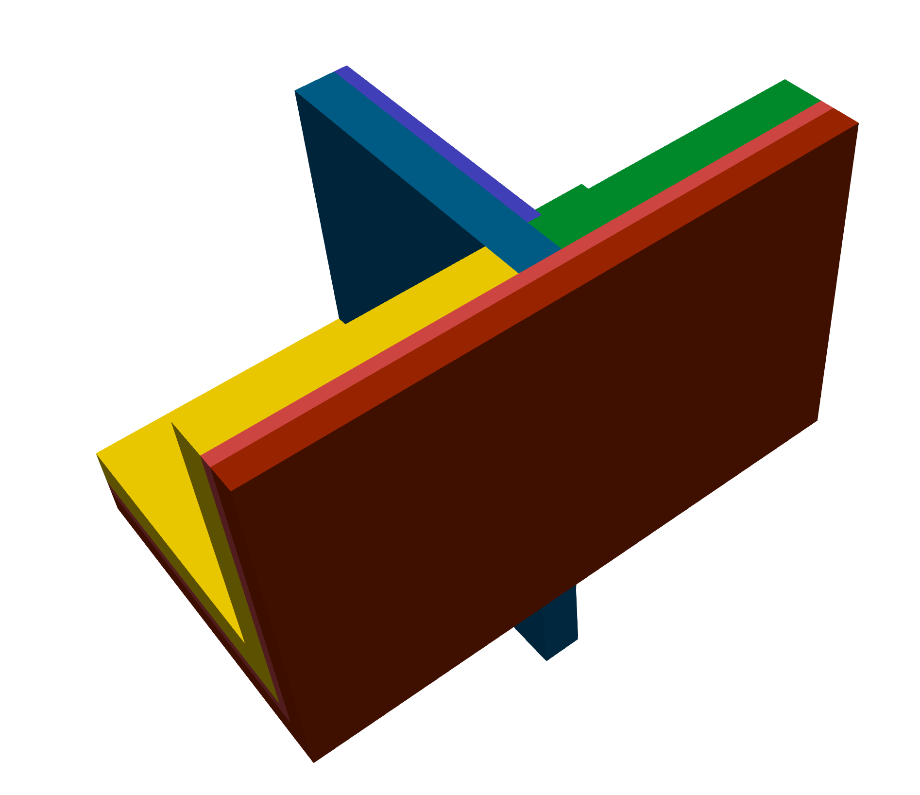
The Figure 4.3 represents the geometry of this benchmark and the domain decomposition by material.

The benchmark was performed on the gaya supercomputer (see Section 10.1). The performance tools integrated into the Feel-toolboxes framework were used to measure the execution time. Moreover, we need to note that we have used here Apptainer with Feel SIF image based on Ubuntu noble OS.

This benchmark was done using feelpp.benchmarking, version 4.0.0

The metrics measured are the execution time of the main components of the simulation. We enumerate these parts in the following:

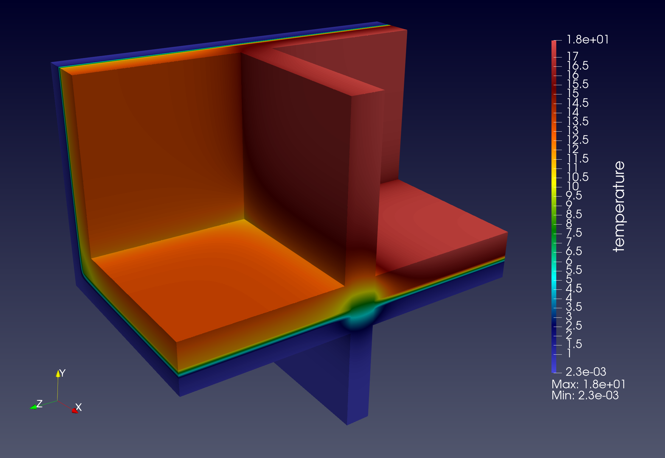
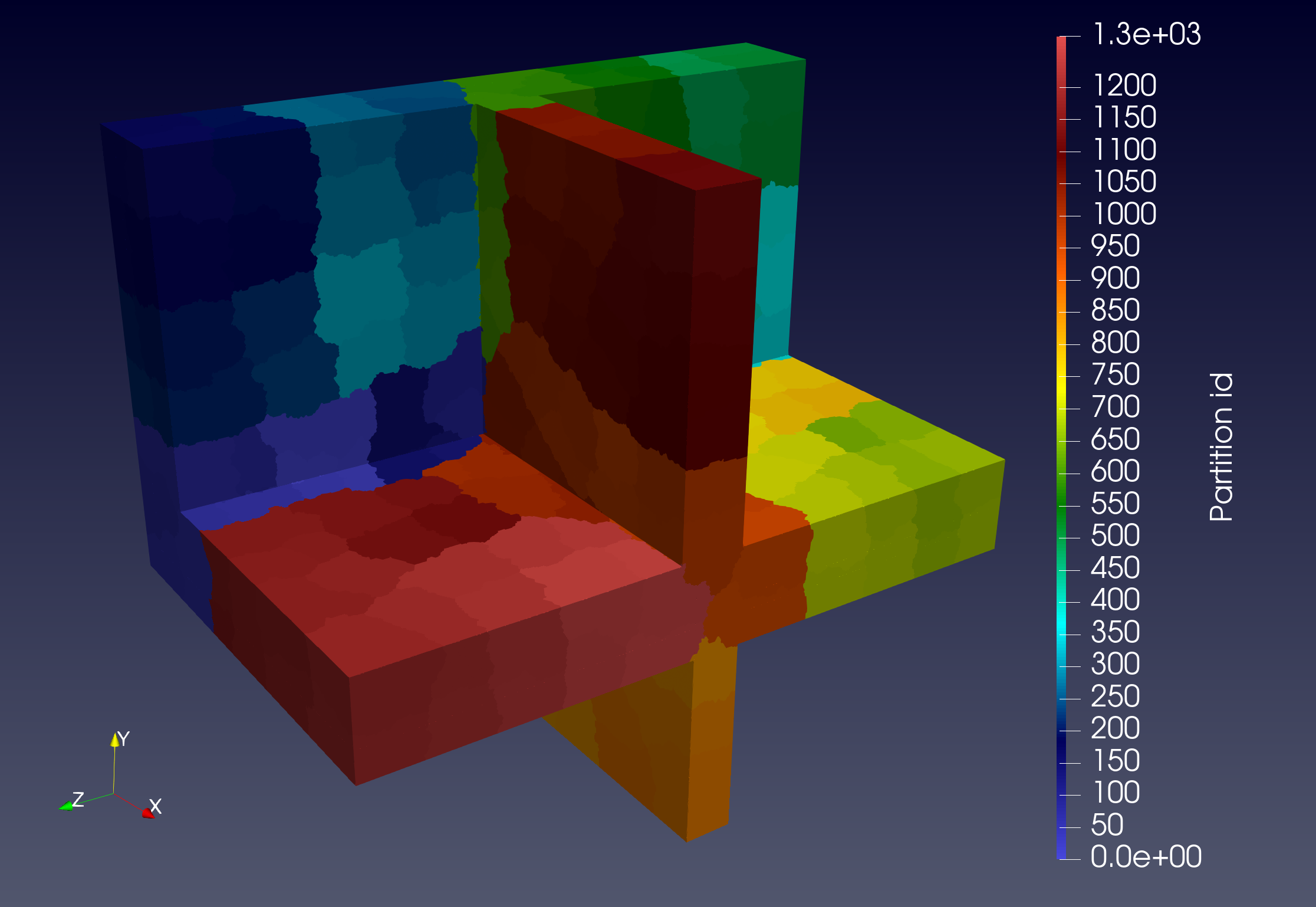
We start by showing in fig. 4.4 an example of numeric solution and mesh partitioning that we have obtained in the simulation pipeline. The partitioning process is considered an offline process here but requires some time and memory consumption. This should be explicitly described in a future work. With fig. 4.5, we have validated the simulation run by checking measures compared to reference values.

The benchmark performance results are summarized in Figure 4.6, Figure 4.7, Figure 4.8 which correspond respectively to choice of the mesh M1, M2 and M3. Moreover, for each mesh, we have experimented with several finite element discretizations called P1, P2 and P3. For each order of finite element approximation, we have selected a set of number of CPU cores. Concerning the mesh M1, considered a coarse mesh, we note that the scalability scaling is not good, especially for low order. This is simply because the problem is too small for so many HPC resources. MPI communications and IO effects are non-negligible. For the mesh M2 and M3, results are better (but not ideal), and we can rapidly see the limit reached by the scalability test. Finally, the fined mesh M3, illustrates the best scalability on this benchmarking experiment. We see a reduction in computational cost by increasing the computation resources. However, due to the fast execution, the time goes fast to the limit.

With these benchmarking experiences, we have also seen that we have some variability in performance measures. Some aspects such as the filesystem and network load, are not under our control, it can explain a part of this (when computational time belongs small locally).

Several challenges were encountered during the benchmarking process:

To conclude, we have realized HPC performance tests of benchmark called thermal bridges. We have realized with success the execution of several simulations on significant resources and demonstrated the validation of Feel framework in the elliptic PDE context. We have also validated the deployment of Feel with container support. Now, we need to provide more refined measures to detect and analyze reasons for performance degradation. And also compare to other software installations, like Spack.